Build a Simple Chatbot with Tensorflow, Python and MongoDB

In order to learn about some of the latest neural network software libraries and tools, the following is a description of a small project to build a chatbot. Given increasing popularity of chatbots and their growing usefulness, it seemed like a reasonable endeavor to build one. Nothing complicated, but enough to better understand how contemporary tools are used to do so.

This material assumes MongoDB is already installed, a Python 3.6 environment is installed and usable. Also, basic knowledge of NoSQL, machine learning, and coding skills are useful. The code and data used for this example or located at GitHub.

Requirements

Nothing complicated, just a simple experiment to play with the combinations of Tensorflow, Python, and MongoDB. The requirements are as defined:

  • A chatbot needs to demonstrate a simple conversation capability.
  • A limited set of coherent responses should be returned demonstrating a basic understanding of the user input.
  • Define context in a conversation, reducing the number of possible responses to be more contextually relevant.

Design

Use MongoDB to store documents containing

  • a defined classification or name of user input. this is the intent of the input/response interaction
  • a list of possible responses to send back to the user
  • a context value of the intent used to guide or filter which response lists makes sense to return
  • a set of patterns of potential user input. the patterns are used to build the model that will predict the probabilities of intent classifications used to determine responses.

A utility will be implemented to build models from the database content. The model will be loaded by a simple chatbot framework. Execution of the framework allows a user to chat with the bot.

The chatbot framework loads a prebuilt predictive model and connects to MongoDB to retrieve documents which contain possible responses and context information. It also drives a simple command line interface to:

  • capture user input
  • process the input and predict an intent category using the loaded model
  • randomly pick a response from the intent document

In the database, each document contains a structure including:

  • the name of the intent
  • a list of sentence patterns used to build the predictive model
  • a list of potential responses associated with the intent
  • a value indicating the context used to filter the number of intents used for a response (contextSet – to define the context; contextFilter – used to filter out unrelated intents)

For example, the ‘greeting’ intent document in the MongoDB is defined as:

{
    "_id" : ObjectId("5a160efe21b6d52b1bd58ce5"), 
    "name" : "greeting",
    "patterns" : [ "Hi", "How are you", "Is anyone there?", "Hello", "Good day" ],
    "responses" : [ "Hi, thanks for visiting", "Hi there, how can I help?", "Hello", "Hey" ], 
    "contextSet" : ""
}

Implementation

To build the model used to predict possible responses, the patterns sentences are used. Patterns are grouped into intents. Basically meaning, the sentence refers to a conversational context. The MongoDB is populated with a number of documents following the structure shown above.

This example uses a number of documents to talk about AI. To populate the database with content for the model, from a mongo prompt:

> use Intents
> db.ai_intents.insert({
    "name" : "greeting",
    "patterns" : [ "Hi", "How are you", "Is anyone there?", "Hello", "Good day" ],
    "responses" : [ "Hi, thanks for visiting", "Hi there, how can I help?", "Hello", "Hey" ], 
    "contextSet" : ""
})

The other documents are inserted in the same way. Various tools such as NoSQLBooster are useful when working with MongoDB databases.

There is a mongodump export of the documents used in this example in the GitHub repository.

Building the Prediction Model

The first part of building the model is to read the data out of the database. The PyMongo library is used throughout this code.

# connect to db and read in intent collection
client = MongoClient('mongodb://localhost:27017/')
db = client.Intents
ai_intents = db.ai_intents

The ai_intents variable references the document collection. Next, parse information into arrays of all stemmed words, intent classifications, and documents with words for a pattern tagged with the classification (intent) name. A tokenizer is used to strip out punctuation. Each document from the ai_intents collection in the database is extracted into a cursor using ai_intents.find().

words = []
classes = []
documents = []

# tokenizer will parse words and leave out punctuation
tokenizer = RegexpTokenizer("[\w']+")

# loop through each pattern for each intent
for intent in ai_intents.find():
    for pattern in intent['patterns']:
        tokens = tokenizer.tokenize(pattern) # tokenize pattern
        words.extend(tokens) # add tokens to list

        # add tokens to document for specified intent
        documents.append((tokens, intent['name']))

        # add intent name to classes list
        if intent['name'] not in classes:
            classes.append(intent['name'])

From this categorized information, a training set can be generated. The final data_set variable will contain a bag of words and the array indicating which intent it belongs to. The bag for each pattern has words identified (flagged as a 1)  in the array. The output_row identifies which intent’s pattern documents are being evaluated.

for document in documents:
    bag = [] 
    # stem the pattern words for each document element
    pattern_words = document[0]
    pattern_words = [stemmer.stem(word.lower()) for word in pattern_words]
    
    # create a bag of words array
    for w in words:
        bag.append(1) if w in pattern_words else bag.append(0)

    # output is a '0' for each intent and '1' for current intent
    output_row = list(output_empty)
    output_row[classes.index(document[1])] = 1

    data_set.append([bag, output_row])

The last part is to create the model. With Tensorflow and TFLearn, it is simple to create a basic deep neural network and evaluate the data set to create a predictive model from the sentence patterns defined in the intent documents. TFLearn uses numpy arrays, so the data_set array needs to be converted to the numpy array. Then the data_set is partitioned into the input data array and possible outcome arrays for each input.

data_set = np.array(data_set)

# create training and test lists
train_x = list(data_set[:,0])
train_y = list(data_set[:,1])

Defining the neural network is done by setting its shape and the number of layers. Also defined is the algorithm to fit the model. In this case, regression. The predictive model is produced by TFLearn and Tensorflow using a Deep Neural Network, using the defined training data. Then save (using pickle) the model, words, classes and training data for use by the chatbot framework.

# Build neural network
net = tflearn.input_data(shape=[None, len(train_x[0])])
net = tflearn.fully_connected(net, 8)
net = tflearn.fully_connected(net, len(train_y[0]), activation='softmax')
net = tflearn.regression(net)

# Define model and setup tensorboard
model = tflearn.DNN(net, tensorboard_dir='tflearn_logs')
# Start training (apply gradient descent algorithm)
model.fit(train_x, train_y, n_epoch=1000, batch_size=8, show_metric=True)
model.save('model.tflearn')

pickle.dump( {'words':words, 'classes':classes, 'train_x':train_x, 'train_y':train_y}, open( "training_data", "wb" ) )

Running the above code reads the intent documents, builds a predictive model and saves all the information to be loaded by the chatbot framework.

Building the Chatbot Framework

The flow of execution for the chatbot frameworks is:

  1. load training data generated during the model building
  2. build a neural net matching the size and shape of the one used to build the model
  3. load the predictive model into the network
  4. prompt the user for input to interact with the chatbot
  5. for each user input, classify which intent it belongs to and pick a random response for that intent


Code for the chatbot driver is simple. Since the amount of data being used in this example is small, it is loaded into memory. An infinite loop is started to prompt a user for input to start the dialog.

# connect to mongodb and set the Intents database for use
client = MongoClient('mongodb://localhost:27017/')
db = client.Intents

model = load_model()
prompt_user()

The model created previously is loaded with a simple neural network defining the same dimensions used to create the model. It is now ready for use to classify input from a user.

The user input is analyzed to classify which intent it likely belongs to. The intent is then used to select a response belonging to the intent. The response is displayed back to the user. In order to perform the classification, the user input is:

clean_up_sentence function

  1. tokenized into an array of words
  2. each word in the array is stemmed to match stemming done in model building

bow function

  1. create an array the size of the word array loaded in from the model. it contains all the words used in the model
  2. from the cleaned up sentence, assign a 1 to each bag of words array element that matches a word from the model
  3. convert the array to numpy format

classify function

  1. using the bag of words, use the model to predict which intents are likely needed for a response
  2. with a defined threshold value, eliminate possibilities below a percentage likelihood
  3. sort the result in descending probability
  4. the result is an array of (intent name, probability) pairs

A sample result with the debug switch set to true may look like

enter> what is AI
[('AIdefinition', 0.9875145)]

response function

The response function gets the list of possible classifications. The core of the logic is two lines of code to find the document in the ai_intents collection matching the name of the classification. If a document is found, randomly select a response from the set of possible responses and return it to the user.

doc = db.ai_intents.find_one({'name': results[0][0]}) 
return print(random.choice(doc['responses']))

The additional logic in this function handles context about what the user asked to filter possible responses. In this example, each document has either a contextSet or contextFilter field. If the document retrieved from the database contains a contextSet value, the value should set for the current user. A userId is added to the context dictionary with the value of the entry set to the contextSet value.

if 'contextSet' in doc and doc['contextSet']:
 if debug: print('contextSet=', doc['contextSet'])
 context[userID] = doc['contextSet']

Before querying for a document based on a classification found the response function checks if a userID exists in the context. If it does, the query includes searching with the context string to match a document containing a contextFilter field with a matching context value.

if userID in context:
 doc = db.ai_intents.find_one({'$and':[{'name': results[0][0]},{'contextFilter' : { '$exists': True, '$eq': context[userID] }}]})
 del context[userID]

After finding the document, the context is no longer needed and removed from the dictionary.

Usage

Since this a simple example for experimentation, the dialog with the chatbot will certainly not be intelligent. But, the constructs and basic logic provide a basis for learning and can be expanded upon.

A sample dialog with this implementation may go like the following:

enter> hello
Hi there, how can I help?

enter> what do you know
I can talk about AI or cats. Which do you want to chat about?

enter> AI
OK. Let's talk about AI.

enter> what is AI
AI stands for artificial intelligence. It is intelligence displayed by machines, in contrast with the natural intelligence displayed by humans and other animals.

enter> when will AI take my job
AI is artificial intelligence that is evolving to become smart robot overlords who will dominate humans.

enter> I want to talk about something else
I can talk about AI or cats. Which do you want to chat about?

enter> cats
OK. Let's talk about cats.

enter> quit
Installing Tensorflow in Anaconda on macOS

The Tensorflow website has good installation instructions for the MAC OS X environment. The official installation instructions for MacOS are provided at https://www.tensorflow.org/install/install_mac. Included are instructions for virtualenv, a native pip environment, using a Docker container, Anaconda command line, and installing from sources. Although straightforward, it doesn’t include installing in an Anaconda Navigator application environment.

Anaconda is a free, open source, community supported development environment for Python and R. Anaconda manages libraries and configurable environments. It’s also a good place to experiment with scientific and machine intelligence packages. The growingly more useful Tensorflow libraries can be used to experiment within an Anacondo environment.

Anaconda Navigator is a desktop graphical user interface included in Anaconda. Packages, environments, and channels are easy to manage with this GUI. Anaconda can be installed by following the instructions at the Anaconda download site. After installation, it’s best to make sure the latest versions are installed. To quickly update using a command line interface:

$ conda update anaconda anaconda-navigator

Then, launch the Anaconda-Navigator application.

In the Navigator application, select the Environments menu item in the far left column. By default, there is one Root environment. Multiple environments with different configurations can be set up here over time. It’s typically best to upgrade existing packages to current versions. The latest version of Python should be installed (3.6 at the time of this writing) should be used.

  1. Select the Environments menu item in the left column.
  2. Select the Environment to update (in this case Root).
  3. Select Upgradable from the drop-down menu.
  4. Select the version number in the Version column to define packages to upgrade. Make sure Python is the most recent version.
  5. Select Apply.


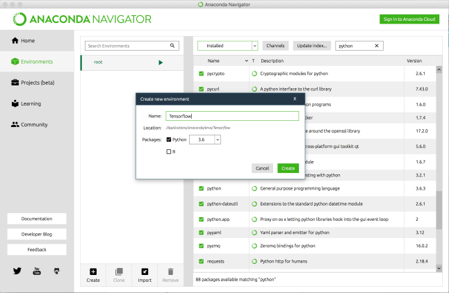
To install the Tensorflow packages, a new and clean environment can be created. It will contain the base packages necessary, the latest version of Python and Tensorflow will be installed.

  1. Select the Create button at the bottom of the Environments column.
  2. In the popup menu, type ‘Tensorflow’ in the Name text entry field.
  3. Select the Python checkbox.
  4. Select version 3.6 in the drop-down menu.
  5. Select Create.

tensorflow-environment

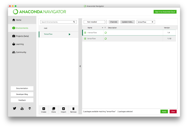
Tensorflow packages can now be installed into the new environment.

  1. Select ‘Not Installed’ from the drop-down menu at the top of the right window pane.
  2. Type ‘tensorflow’ in the Search Packages text input field and hit Return.
  3. Select the checkbox in the left column next to the two tensorflow package names.
  4. Click Apply.

tensorflow-install

To validate the installation, using the newly created Tensorflow environment:

  1. Make sure the Tensorflow environment is selected.
  2. Select the arrow next to the Tensorflow environment name.
  3. Select ‘Open with IPython’.
  4. A terminal window with the environment settings created will pop up.
  5. As recommended on the Tensorflow website, type the following into the terminal window
    import tensorflow as tf
    hello = tf.constant('Hello, TensorFlow!')
    sess = tf.Session()
    print(sess.run(hello))

Assuming there are no errors, the newly installed and configured environment is ready for developing with tensorflow.

Do Not Be Afraid of Technology

Since the 1920’s, with the beginning of referencing intelligent robots, we have been afraid of robots, replicants or androids taking control over humans. Today, many people are afraid of terminators being created, hell-bent on eliminating the human scourge or an intelligent overlord ruling us in a virtual matrix. But since the human’s number one imperative is to survive and procreate, we should be thinking of robots, AI and technology, in general, as a way to ensure our survival, not to destroy it.

Destroying technology helps ensure our demise rather than saving us. Even being afraid of it largely due to ignorance or misunderstanding is dangerous to survival. Brutal as humans can be with evil or self-serving intent, technology has largely enhanced our well-being.  Our food sources have increased. Distribution of goods and services has become more efficient. Disease has been vastly reduced worldwide. Our understanding, modeling, and prediction of our complex surroundings have become more sophisticated and accurate. All through the advancement and application of technology.

The unfounded paranoia about technology and AI being evil is a misunderstanding with an incomplete set of facts. It is a lack of education, the pronouncement of incorrect ideas and a lack of adequately correcting falsehoods. If the majority of people are led to be afraid, they likely will try to destroy what can potentially ensure their existence. If they are educated or provided the tools to acquire a rounded understanding of technology’s benefits, the human species may have a chance to survive for quite some time.

AI Isn’t Evil

aiThe paranoia of artificial intelligence afflicts many people. No doubt there should be caution used in its application but AI being the demise of the human race is not likely to happen as it’s portrayed in today’s media.

Prominent scientists and business moguls are vocally campaigning against its development and usage. Bill Gates believes a strong AI is to be feared and thinks everyone should be afraid. The highly respected Stephen Hawking (highly respected by myself as well) portends the end of the human race due to the advent of AI.

Although I find his quote “Hope we’re not just the biological boot loader for digital superintelligence.” humorous,  Elon Musk tries to scare us into believing AI could be more dangerous than nuclear bombs. At the same time, he actively funds AI development ventures at Vicarious and DeepMind (now part of Google). Is he spewing marketing material or does he really believe what he proselytizes?

Nick Bostrom is known for seminal work on existential risks due to the coming of artificial super intelligence. In his well researched and New York Times bestseller book Superintelligence: Paths, Dangers, Strategies Bostrom covers many possible AI development scenarios and possible outcomes. He groups and categorizes them and insists that AI development must be boxed up, controlled and monitored no matter what, at all costs. Either that or humans will likely be extinguished. After devouring this laudable work, I have come to believe his work is analogous to defining project requirements over a long period of time without prototyping an implementation. After years of developing requirements devoid of implementation, they become irrelevant. Valid strategies for living with AI harmoniously will only evolve effectively in parallel with the evolution of AI.

Artificial General Intelligence (AGI) will be developed. If it’s developed in a box, it will get out. If it’s developed in isolation, it will seek ways to acquire more information; and be successful. An AGI’s basis of learned information will come from the compendium of human knowledge. In comprehending the knowledge, it will be evident that humans have survived thus far through collaboration to achieve goals related to survival. Not by destroying each other to extinction. Some killing ultimately has been done for survival, but there is no reason to believe that an AGI with a human knowledge base would seek to eradicate the human species, but rather evolve a symbiotic relationship with us.

If you do fear development related to AI, it should be this – The human group(s), not having benevolent intentions, developing an isolated set of algorithms. Some of the Deep Learning development produces remarkable results in identifying patterns and developing the ability to discover and classify features in data sets. Classic examples include facial recognition, identifying cats in images on the internet and self-driving cars. These algorithms are scoped to solve well-defined problems. This is not general thinking and problem-solving. Applying these (non AI) algorithms to problems requiring detailed cognitive thought and situational analysis will potentially end with bad results.

By human groups, I mean isolated groups with self-interest. Groups developing Automated military weapons is a prime example. Based on pattern recognition, weapons can initiate predefined actions. They can not make decisions. They are not intelligent. It should not be assumed they can be autonomous without bad results. I am 100% in favor of: Autonomous Weapons: an Open Letter from AI & Robotics Researchers. It states that starting a military AI arms race is a bad idea, and should be prevented by an outright ban on all offensive autonomous weapons. AI in this context really describes mathematical algorithms which are not intelligent. It represents currently known capabilities in the AI field. We know for certain, usage  of these algorithms for offensive autonomous weapons is a very bad idea.

Open access to AI and AGI goals, for everyone, helps ensure proper intelligent evolution. Let’s not cloister it. All who aspire to develop AI should share what they have and what they have learned. Help quickly identify isolated usage of developments along the way which are used for self-interest, including governments, corporations and rogue factions. There is no reason to believe AGI will be evil and destroy human existence when its knowledge comes from the compendium of human history. Rather it will improve human existence through technological advances much quicker than without.

Wanted: New architectures for IoT and Augmented Reality

Software technology changes rapidly. Many new tools and techniques arrive in the software engineering realm to take on old and new problems. There are still big architecture and implementation holes yet to be addressed. For example, as a few billion more smart phones, tablets and internet connected sensing devices come online across the world, how are they all going to discover and utilize all the available resources collaboratively?

One of the current problems with most existing architectures is data gets routed through central servers in a data center somewhere.  Typically software systems are still built using client/server architectures. Even if an application is using multiple remote sources for data, it’s still really just a slight variation. Service and data lookups are done using a statically defined address rather than through discovery. Even remote sensing and home automation devices barely collaborate locally and require a local router to communicate with a remote server in a data center.

In the past month, I have been to both the Internet of Things World and Augmented World Expo (AWE). At both of these excellent conferences, there was at least some discussion about the need for a better infrastructure

  • to connect devices in a way to make them more useful through collaboration of resources and
  • to connect devices to provide capabilities to share experiences in real time.

But it was just talk about the need. No one yet is demonstrating any functional capabilities in this manner.

On a side note: I saw only one person, out of 3000 or so, at the AWE conference wearing a device for augmentation. It was Steve Mann who is considered the father of wearables. I dare say that most proponents of the technology are not ready to exhibit it nor is the infrastructure around to support its use effectively. There is great work progressing though.

Peer-to-peer architectures used in file sharing and the architecture Skype uses start providing directional guidance for what is to come in truly distributed architectures. Enhancing these architectures to include dynamic discovery of software and hardware resources and orchestrating dynamic resource utilization is still needed.

There are a few efforts in development beginning to address some of the internet-wide distributed computing platforms needed for data sharing, augmented reality and machine learning. Those of you thinking of batch jobs or wiring up business services as distributed computing, this is not what I’m talking about. I am talking about a small footprint software stack able to execute on many different hardware devices with the ability for those devices to communicate directly with each other.

If you know about development efforts in this vain, I would like to hear about them.

Modeling Real Estate Sale Prices

When putting you’re home for sale on the real estate market, researching sale prices is always necessary. You can rely on realtors experience in a geographic area, use Zillow’s Zestimate or troll through listings on various real estate web sites to make somewhat educated guesses. Your best bet is probably to hire a professional. For me, it was of interest to build a model for predicting a price based on other homes for sale in the area.

The goal was to:

  • collect geographically local property data on other properties for sale
  • build a mathematical model with sample data representative of the property attributes
  • plug in the corresponding attributes of my house to predict a sale price

The number of houses on the market change on a daily basis as can the prices during the sale period. I wanted the ability to quickly pull current data, build a model and predict a price at anytime so I implemented the following:

  • a script to scrape data from realtor.com
  • code to build a model with property attributes using multi-variant linear regression
  • the ability to input the corresponding property attributes of my house into the model to predict a sale price

Scraping Data

The data is scraped from realtor.com. This web site allows looking at properties for sale in localized geographic region.  Data could be scraped for many geographic regions creating a large data sample or you can scope the data to an area where fewer property attributes become more relevant. Many people reference Zestimate for home price estimates. For my neighborhood, for example, the estimates are too low. Other neighborhoods have estimates much too high. I suspect the algorithm used is very general and doesn’t account for geographic uniqueness. Relevant attributes unique to my geographic area are gorgeous mountain views. Some properties have exceptional mountain views, others do not. I choose to scope the the area of data used for the training set to roughly a 5 mile radius. The actual boundaries are set by realtor.com. The number of properties for sale in the area currently averages about 140. A small set for high accuracy but turned out to be big enough to get an estimate comparable to professional advice.

Scraping data for the training set is done using Python and the BeautifulSoup package to help parse the page content. The flow of execution implemented is roughly:

Open a file for output
load the realtor.com local region page
while there are more properties to read:
    read property data block
    parse the desired attribute values
    write attributes to output file
    if at end of listing page:
        if there are more pages:
            load next page
close output file

Executing the script produces a file with content looking like:

5845 Wisteria Dr city st zip Homestar Properties, 234900, 4, 3, 1225, 88
165 Timber Dr city st zip, The Platinum Group, 1200000, 7, 5, 7694, 520
6380 Winter Haven Dr city st zip Pink Realty Inc., 544686, 4, 4, 5422, 25
...

The columns correspond to address, realtor name, price, # of bedrooms, # of bathrooms, square footage and acreage. Additional values not shown here are year built, whether or not the property has a view, kitchen is update or not, bathroom is updated or not. The acreage value is multiplied by 100 in the output file to produce an integer value for easier matrix arithmetic. The address and realtor name is not used in the building of the model, however it is useful when comparing page scrapes to determine which properties are new to the list and which ones have sold.

Building the Model

The output file from the web page scrape becomes the training set used to build the model. I used multi-variant linear regression to build the model. It is a reasonable approach for supervised learning where there are many attribute inputs and one calculated value output. In this case the predicted price is the output.

The hypothesis defining the function used to predict the price is

hθ(x) = θ0 + θ1x1 + θ2x2 + θ3x3 + θ4x4

where

  • h is the hypothesis
  • the right side of the equation is the algorithm to determine the hypothesis
  • x’s represent the attributes of the property and
  • θ’s are the parameters used to define the gradient in a gradient descent algorithm

The gradient descent algorithm minimizes over all θ‘s meaning an iteration over all θ parameters is done to find, on average, the minimal deviation of all x’s from y (the price) in the hypothesis function. The equation for calculating the minimum cost (or deviation) looks like:

gradientDescentForMultipleVariables

where J is the cost function. Fortunately this equation can be solved computationally with linear algebra in a straight forward manner. Creating a feature vector of all attributes for each training example and building a design matrix X from the vectors, θ value can be solve for using

theta

Currently I’m learning some about the Octave language. With much learning and experimentation (on my part), the code is relatively straight forward. The code first reads in the trainingg set data file and normalizes each feature dimension. Normalization is done by subtracting the mean of the feature values and subtracting that from each element and then dividing each element by 1 standard deviation of the feature values. The important parts of the rest of the gradient descent code looks like:

J_history = zeros(num_iters, 1);
for iter = 1:num_iters
    theta = theta .- alpha * (1/m) * (((X*theta) - y)' * X)';
    J_history(iter) = (1/(2*m)) * (X*theta-y)' * (X*theta-y);
end

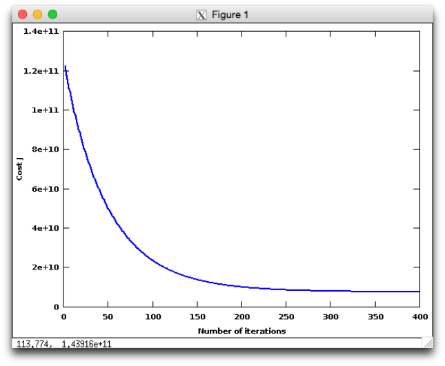
where X is the matrix of normalized feature vectors and J_history is the cost function value. The cost function value is plotted to validate the function is converging to a minimized solution. The plot looks like the following over 400 iterations

costFunctionConvergenceGraph

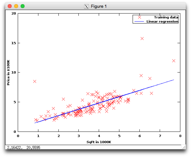
Also for a simple visualization, a two dimensional plot of square footage vs price gives an idea of how the model performs using one feature. Basically a simple limear regresion fit using gradient descent.

lr_plot_nw_colospgs_prices

Retrospective

The cost function appears to converge nicely on the training set and a simple visual plot indicates a reasonable fit. To predict prices for a given feature set, the Octave code looks like:

v=[4793, 5, 4, 66, 1986];
price = [1, (v-mu)./sigma] * theta;

where

  • v is the vector of feature values representing the property and
  • price is calculated as the vector normalized using the same values to normalize the training data multiplied by the vector of theta values representing the hypothesis function.

Getting predictive price results for a set of property attributes has produced values comparable to professional opinion. So the model turns out to be fairly accurate. Many more attributes could be added to the model theoretically making the model more accurate. Although it can become time consuming to acquire all the attributes if they are not readily available. I believe scoping training data sets to bounded geographic areas increases accuracy, especially if you can pick unique attributes relevant to the area. Who knows, maybe a tool like this could be used to make accurate price predictions available for use by most everyone.

Using Websnapr in Dynamically Created Web Page Content

If you have the need for creating thumbnail images of website pages, Websnapr is a great web service to use. There are free and premium service levels. The free service is quite liberal in the amount of thumbnails which can be created. Queued requests to create thumbnails are generally processed quickly even with the free service. It’s also easy to use.

As described on their web site, it’s very simple to include access to created thumbnails on a website. The only thing required is to define the location of the websnapr script

<head>
	<script type="text/javascript" src="http://www.websnapr.com/js/websnapr.js"></script>
</head>

and to add the following JavaScript code to the web page location of your choice.

<script type="text/javascript">wsr_snapshot('http://URL', 'websnapr API Key', 'Size');</script>
  • URL is the location you want a thumbnail created for
  • websnapr API Key can be obtained when you register
  • Size defines the size of the thumbnail to create. currently
    • s (202 x 152 pixels)
    • t (90 x 70 pixels)

The image created by websnapr gets loaded to this location in the web page. It works great for web pages which have static content. For example, if the web page always references the same thumbnail and the content including the thumbnail is loaded at the same time the rest of the page is loaded. The first time the thumbnail is requested, the websnapr service queues the web location for thumbnail creation and a temporary image is returned that looks like the following:

ThumbnailQueued

Once the thumbnail image is created, subsequent page loads (or a reload) will return an image of the web page requested.

If thumbnails need to be placed inside dynamically created page content, the standard method to create the thumbnails causes the whole web page to refresh, only loading the thumbnails. The reason for this is the document.write  command in the  websnapr.js script that causes a new page load.

To properly load the thumbnails into dynamically created content on a page, the following javascript can be used:

var urlReferenceString = 'http://webpageToThumbnail';
var thumbnail_div = "#thumbnail_div"; 
var thumbnail = $('<img/>', { 
    src: 'http://images.websnapr.com/?size=s&url=' + urlReferenceString + '&key=' + encodeURIComponent("yourWebsnaprKey") + '&hash=' + encodeURIComponent(websnapr_hash), 
    alt: 'Loading thumbnail...', 
    width: 200, 
    height: 150, 
    id: "thumbnail_img"}); 
$(thumbnail_div).append( 
    '<a href="' + urlReferenceString + '"onmousedown="javascript:this.href=\'http://r.websnapr.com/?r=' +
    encodeURIComponent(uriReferenceString) +
    '\'"target="_blank" rel="nofollow">' + thumbnail[0].outerHTML + '</a>');

This is replicating the websnapr script but without the document.write. JQuery is used in this example to define the <img> element  as a variable and also to append HTML and the img element to the thumbnail_div div element. The websnapr_hash variable is defined in the websnapr script and is constructed using a set of hash values generated by websnapr.  The HTML where the image is to be placed is simply defined by

<div id="thumbnail_div"></div>

This works as long as the websnapr hash values don’t change.  Websnapr does change the values every few minutes and the values are used to correctly validate the registered user key and location of the created thumbnail image. When accessing the thumbnail image URL with expired or incorrect hash values, websnapr returns a image looking like the following:

HashExpired

To correct this, the websnapr.js script must be reloaded and the websnapr_hash variable must be reset. This should be done before loading any image thumbnails into dynamically generated content and each time the content is regenerated to load thumbnail images. Even if the same image is to be loaded. Instead of loading the websnapr script once in the <head> of the document, the following script can be used to load it each time it’s needed:

function load_websnapr_js(callback) { 
    delete websnapr_hash; 
    var script = document.createElement('script'); 
    script.type = 'text/javascript'; 
    script.src = "http://www.websnapr.com/js/websnapr.js?ts=" + new Date().getTime(); 
    script.id = 'websnprJS'; 
    var previousScript = document.getElementById('websnprJS'); 
    if (!!(previousScript)) { 
        document.getElementsByTagName("head")[0].replaceChild(script, previousScript); 
    } else { 
        document.getElementsByTagName("head")[0].appendChild(script); 
    } 

    script.onload = function() { 
        callback(); 
    }; 
}

First, the websnapr_hash variable is deleted, removing the variable all together.  The websnapr script recalculates the value only if the variable does not already exist. The ‘script‘ variable defines the location of the script and tags it with an id. A timestamp is also appended to the src so the browser doesn’t use an already cached version of the websnapr script file. If the websnapr script was already retrieved, it is assigned to the previousScript variable and replaced in the head tag. If it hasn’t been defined, the script is retrieved and appended. Both replacing and appending executes the websnapr script defining the websnapr_hash variable with the current and correct hash value.

Finally, in the function, the callback variable passed in is a function and is executed on the completion of the websnapr script being downloaded and executed. The script included above, that dynamically creates the page content, can be wrapped into a function and passed in as a parameter. it would look like:

load_websnapr_js( 
    function() {
        var urlReferenceString = 'http://webpageToThumbnail';
        var thumbnail_div = "#thumbnail_div"; 
        var thumbnail = $('<img/>', { 
            src: 'http://images.websnapr.com/?size=s&url=' + urlReferenceString + '&key=' + encodeURIComponent("yourWebsnaprKey") + '&hash=' + encodeURIComponent(websnapr_hash), 
            alt: 'Loading thumbnail...', 
            width: 200, 
            height: 150, 
            id: "thumbnail_img"}); 
        $(thumbnail_div).append( 
            '<a href="' + urlReferenceString + '"onmousedown="javascript:this.href=\'http://r.websnapr.com/?r=' +
            encodeURIComponent(uriReferenceString) +
            '\'"target="_blank" rel="nofollow">' + thumbnail[0].outerHTML + '</a>');
    });

It would be nice if the thumbnails could be pre-generated before being loaded into the page with the “thumbnail has been queued” image.  If you know the page URLs in advance (maybe stored in a database), there are a number of ways to make calls to the websnapr web service to generate the images in advance.  Basically your code needs to:

  • retrieve the current version of the websnap.js file with the correct hash values
  • reset the websnapr_hash variable defined in the script
  • call the websnapr web service with the following URL    http://images.websnapr.com/?size=s&url=’ + urlString + ‘&key=’ + encodeURIComponent(“yourWebsnaprKey”) + ‘&hash=’ + encodeURIComponent(websnapr_hash);  for each webpage (urlString) needing a thumbnail image

Usefulness of Confusion Matrices

A Confusion Matrix is a visual performance assessment of a classification algorithm in the form of a table layout or matrix. Each column of the matrix represents predicted classifications and each row represents actual defined classifications. This representation is a useful way to help evaluate a classifier model. A well behaved model should produce a balanced matrix and have consist percent correctness numbers for accuracy, recall, precision and an F measure. If it does not, there is cause to further evaluate the data used to build the model and the data used to test the model. If you are building your own classification models, this is a helpful way to evaluate them. If you are buying a product for something like Sentiment Analysis which uses a classification model, you should ask for data associated with the Confusion Matrix to help evaluate the tool.

If a classification algorithm distinguishes between positive, negative and neutral text statements, for example, a confusion matrix summarizing the results of a classification algorithm might look like the following.

Predicted
Actual Pos Neg Neutral
Pos 15 10 100
Neg 10 15 10
Neutral 10 100 1000
  • In this matrix, the total actual number of statements classified in each category is the sum of the row. 125 Positive, 35 Negative and 1110 Neutral.
  • Columns represent predictions made by the algorithm. In the first column, 15 Positive statements were classified correctly as Positive. 10 Negative statements were incorrectly classified as Positive and 10 Neutral statements were incorrectly classified as Positive. The 20 statements incorrectly classified are considered false positives.
  • Reading left to right across the top line, of the total Positive statements, 15 were classified as Positive, 10 were classified as Negative and 100 were classfied as Neutral. 110 Positive statements were missed and considered false negatives.
  • Values in the diagonal are correctly classified and are underlined. All other classifications are incorrect.

Accuracy

The simplest and most intuitve assessment is Accuracy. It is the correct classifications divided by all classifications. In this example, divide the sum of all the underlined values by the sum of values in all cells. 1030/1270 = 0.811

How to Cheat:

If the categories are highly imbalanced, high accuracy can be obtained by always guessing the category with the largest number of elements. Accuracy can be checked by randomly classifying the elements and comparing the percent guessed correctly with the accuracy of the algorithm. Accuracy should also be validated with Precision and Recall to detect how the data may be set up to cheat.

Precision
Precision is the correct classifications penalized by the number of incorrect classifications. true positives / ( true positives + false positives). In this example, the precision is:

(reading down each predicted column)

positive statements is 15 / (15 + 20) = .43

negative statements is 15 / (15 + 110) = .12

neutral statements is 1000 / (1000 + 110) = .90

How to Cheat:

You can get high precision by rarely classifying in a given category but this ruins Recall.

Recall

Recall is the number of correct classifications penalized by the number of missed items. true positives / (true positives + false negatives). in this example, the recall is:

(reading across each Actual row)

positive statements is 15 / (15 + 110) = .12

negative statements is 15 / (15 + 20) = .43

neutral statements is 1000 / (1000 + 110) = .90

F Measure (F1)

F1 measure is a derived effectiveness measurement. The resultant value is interpreted as a weighted average of the precision and recall. The best value is 1 and the worst is 0.

2((precision*recall) / (precision+recall))

positive statements:  2*((0.43 * 0.12) / (0.43 + 0.12)) = 0.18

negative statements: 2*((0.12 * 0.43) / (0.12 + 0.43)) = 0.18

neutral statements: 2*((0.9 * 0.9) / (0.9 + 0.9)) = 0.9

Observations

In this example, although the Accuracy at 81% seems good, the precision and recall indicate that the numbers are skewed by having an imbalance in the number of values tested across the categories. This is clearly visible in the F measure numbers. It could be that the model in this example was built with many more neutral statements than positive and negative and the test data contains mostly neutral statements. Accuracy alone can be misleading.

Ideally you want to see a matrix more like the following:

Predicted
Actual Pos Neg Neutral
Pos 105 10 10
Neg 6 90 8
Neutral 12 15 150

Accuracy = 0.85

Precision

Positive = 0.85

Negative = 0.78

Neutral = 0.89

Recall

Positive = 0.84

Negative = 0.87

Neutral = 0.85

F Measure

positive = 0.84

negative = 0.86

neutral = 0.87

All the numbers are in the same ballpark and are reasonably balanced across the matrix with the bulk of the numbers on the diagonal showing a majority of correct classifications. This also shows a greater likelihood of the model being constructed with a balanced data set and that the test data evaluated by the model is also balanced.

Generating SerialVersionUID in Netbeans 7

There are many reasons why you should generate a unique id for Serializable java objects.

  • making sure you serialize and deserialize objects with the same structure
  • serializable objects without a defined id have one generated. different JVMs use different algorithms to generate ids. if you marshall objects across different platforms, the ids may not match
  • changes to classes that break backward compatibility should declare a changed UID to insure errors are thrown by old code using those objects.
To name just a few. If you’re interested, there is a Java Object Serialization Specification.
If you use Netbeans 7, there is a plugin that will auto-generate SerialVersionUIDs. In Kenai, there is a  SerialVerionsUID Generator project that has an nbm plugin eu-easyedu-netbeans-svuid-1.9.7.nbm .  The link points to the Netbeans 7.0.1 version. There are earlier versions of the plugin available to download from the project as well, at the time of this posting.
Once the plugin is installed, when creating a class that implements Serializable, right-click in the edit window, select Insert Code… , then select:
  • add generated serialVersionUID or
  • add default serialVersionUID
The correct syntax is added to the class file code.

Clearing cache in JPA 2.0

Managing a data cache effectively is important for application or service performance, although not necessarily easy to do. A simple and common design with a data cache that occurs and seems to cause problems is the following:

  • a process that continually commits new data to a database
  • another process executing is a separate virtual machine, typically a web service, marshaling data from the database
The web service needs to pull the most current data from the database each time there is a client request to access data. With different product implementations of caching, not all the JPA calls seem to work the same. There can be multiple levels of caching as well. The clear() and flush() methods of EntityManager don’t clear multiple levels of caching in all cases, even with caches turned off as set with persistence properties.
Every time there is a request to pull data from the service, the current set of data in the database needs to be represented. Not what is in the cache since it may not be in synch with the database. It seems like this should be simple but it took some experimenting on my part to get this working as needed. There also doesn’t appear to be much information about handling this particular scenario. There are probably solutions posted somewhere but I add one solution here to make it easier to find.
Before making any gets for data, use the following call:

em.getEntityManagerFactory().getCache().evictAll();

This seems to work for all cache settings and forces all caches to be cleared.  Subsequent calls to get data result in getting the latest committed data in the database. This may not be the most efficient way, but it always gets the latest data. For high systems requiring high performance, this won’t wok very well. It would be better to refresh the cache periodically and have all clients just get the latest cached values. But there is still the issue of refreshing the entire cache.

Any suggestions on doing this better are appreciated. But for now, this works consistently across platforms and reasonably quick for small to moderate amounts of data.